In Part 2, we saved the Ziggy nodes from the “Loop of Death.” They were now happily scanning the street, generating thousands of logs, and uploading them to my server.
Success, right? Not quite.
I had solved the collection problem, but I had created a storage nightmare. Within a week, I had 140MB of raw CSV files. My initial backend strategy was crude: simply append every new upload to a single master.csv file.
When I tried to load this into Grafana, the Raspberry Pi 5 choked. Parsing a massive text file line-by-line every time I refreshed the dashboard wasn’t just slow; it was crashing the server.
I needed a real database. I needed SQLite.
The Challenge: “Ghost Dates” and Time Travel
Migrating to a database should have been easy, but looking at the raw data revealed a disaster. Because the Ziggy nodes sometimes booted without Wi-Fi (and thus no NTP time sync), thousands of records were stamped with default dates like January 1st, 1970 or January 1st, 2000.
If I imported these “as-is,” my analytics would show cars driving past my house 50 years ago.
I couldn’t just delete them—the relative time stamps (e.g., “2 hours after boot”) were accurate, even if the year was wrong. I wrote a custom “Time Shift” algorithm in Python to detect these “Ghost Dates” and transport them to the present day.
The Code: Fixing the Timeline
This function detects if a timestamp is from a “Ghost Year” (1970 or 2000), calculates how long the device had been running since that fake start date, and adds that duration to my real target start date (Nov 15, 2025).
Python
# The "Real" date the logs started (Time Shift Target)
TARGET_START_DATE = datetime.datetime(2025, 11, 15, 0, 0, 0)

def apply_time_shift(bad_dt):
    """
    Takes a timestamp from 1970 or 2000 and shifts it to 2025.
    Preserves the relative 'uptime' of the scan.
    """
    # 1. Identify the 'Ghost' Base (Factory Default Time)
    if bad_dt.year == 2000:
        ghost_base = datetime.datetime(2000, 1, 1, 0, 0, 0)
    elif bad_dt.year == 1970:
        ghost_base = datetime.datetime(1970, 1, 1, 0, 0, 0)
    else:
        return bad_dt # Unknown error, return as-is

    # 2. Calculate the Delta (Time Since Boot)
    time_since_boot = bad_dt - ghost_base

    # 3. Apply Delta to Reality
    return TARGET_START_DATE + time_since_boot
This logic recovered over 15,000 data points that would have otherwise been deleted as “garbage.”
The Challenge: “Dirty” Data
The second issue was file corruption. Some legacy logs had trailing commas, pushing the column count from the expected 7 to 8, 9, or 10. This caused the database import to fail.
I wrote a “Tail Trimmer” routine. It inspects every line before import, detects empty trailing fields, and snips them off. If the fields aren’t empty (meaning a device name like “iPhone, Red” got split), it intelligently merges them back together.
The Code: The Tail Trimmer
Python
# Remove empty strings from the end of the list until we hit data
original_len = len(parts)
while len(parts) > EXPECTED_COLUMNS and parts[-1].strip() == '':
    parts.pop()

# If we still have too many columns, it's a split ID (e.g. "Smith, John")
if len(parts) > EXPECTED_COLUMNS:
    # Merge the middle columns back into the Device ID field
    merge_count = len(parts) - EXPECTED_COLUMNS
    merged_id = ','.join(parts[2 : 2 + 1 + merge_count])

    # Reconstruct the row with the repaired ID
    final_row = [parts[0], parts[1], merged_id] + parts[2 + 1 + merge_count:]
The Result: The “Hybrid” View
With the data cleaned and indexed in SQLite, queries that used to take 30 seconds now take 10 milliseconds.
But there was one final hurdle: Grafana.
- Grafana Graphs demand time as a Number (Unix Epoch Milliseconds).
- I (The Human) demand time as Text (ISO 8601 String) so I can read it.
Rather than storing the data twice, I created a SQL Virtual View. This acts as a translation layer. It calculates the Epoch on the fly for the machine, while passing the readable text through for me.
SQL
CREATE VIEW grafana_view AS
SELECT
  -- For the Machine: Calculate Epoch Milliseconds on the fly
  strftime('%s', timestamp_utc) * 1000 as time_epoch,

  -- For the Human: Pass the readable text string
  timestamp_utc as human_time,

  -- The Data
  addr, device_id, rssi, security
FROM ble_logs;
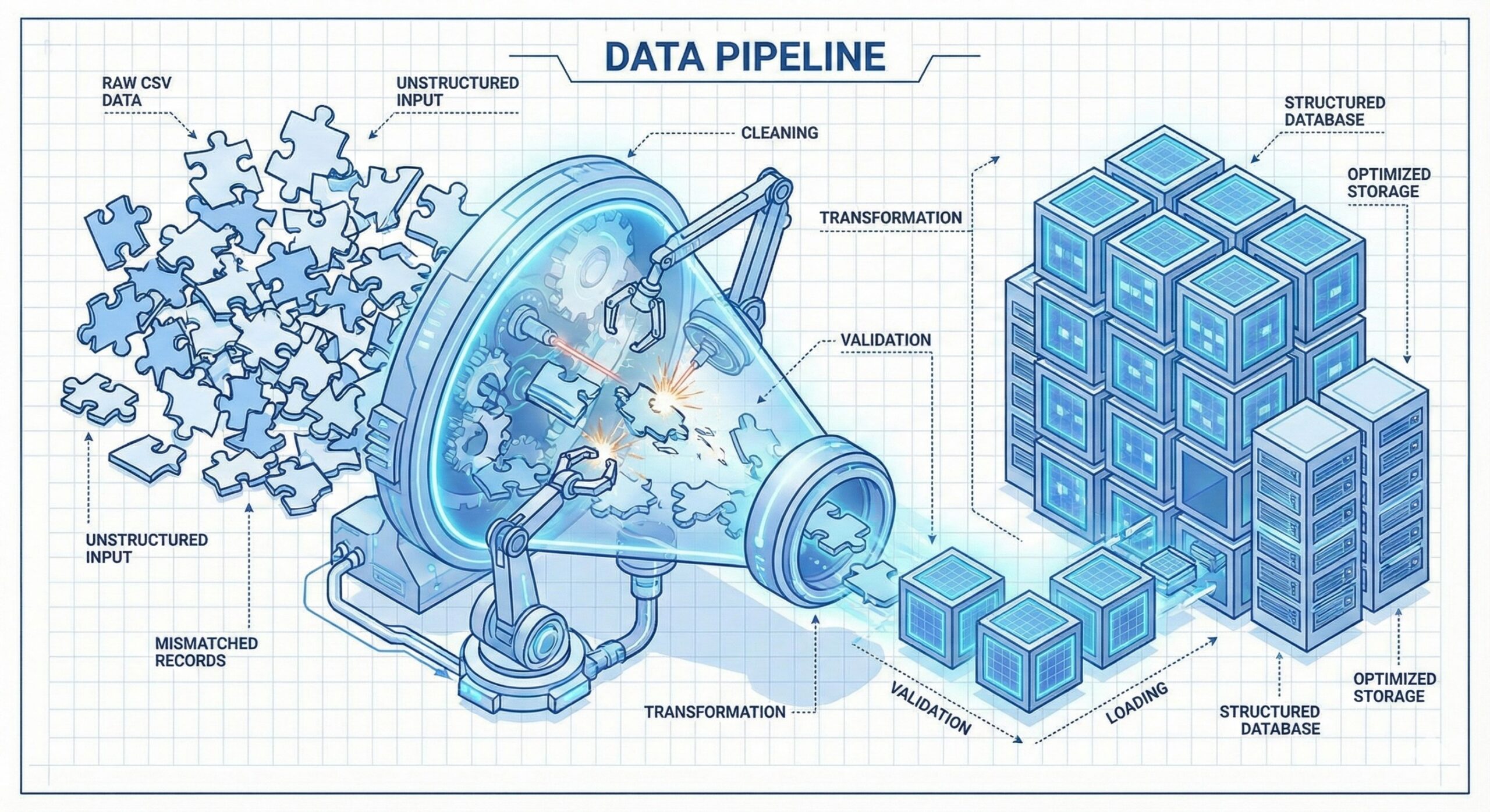
Now, my backend is no longer a fragile pile of text files. It is a robust, self-repairing ETL (Extract, Transform, Load) pipeline that turns raw radio noise into structured intelligence.
Next up: Visualizing the Invisible – Building the Pattern-of-Life Dashboard.