In Part 3, we built a robust backend that could ingest, clean, and store millions of Bluetooth logs. We had the data, but it was sitting in a dark, cold SQLite database file.
Looking at a database cursor is like looking at the Matrix code. You know the woman in the red dress is there, but you have to squint to see her.
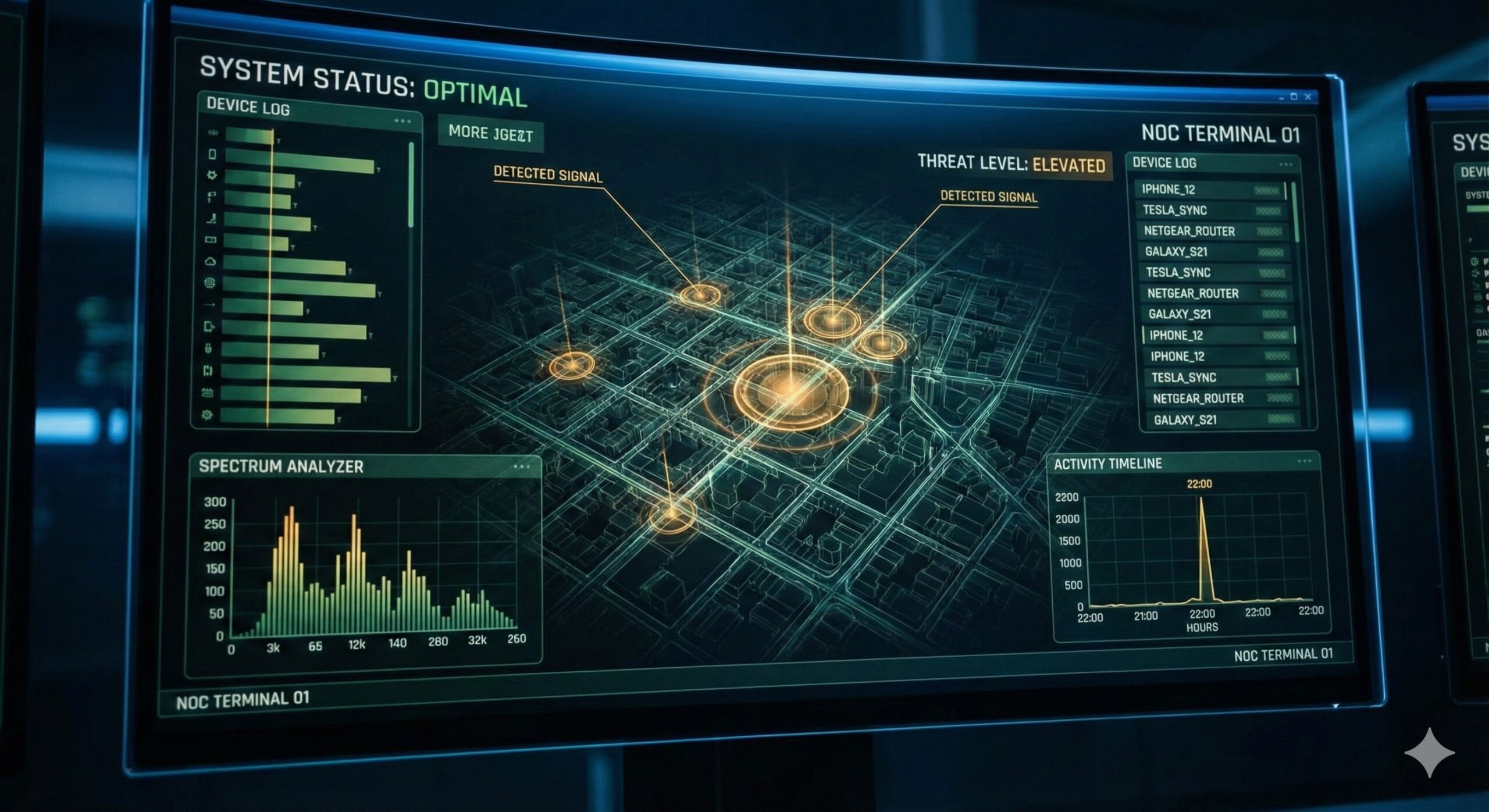
I didn’t want to squint. I wanted a “Mission Control” screen. I wanted to look at a monitor and instantly know: Is the street busy? Who is parked outside? Is that specific delivery truck back again?
To do this, I used Grafana.
The Bridge: The SQL View
Grafana is amazing, but it can be picky. It loves time-series data served as Unix Epochs (numbers), but I prefer reading ISO Strings (text).
Rather than fighting Grafana, I gave it exactly what it wanted using the “Virtual View” strategy we built in Part 3.
SQL
CREATE VIEW grafana_view AS
SELECT
  -- For Grafana: Mathematical Time (Epoch Milliseconds)
  strftime('%s', timestamp_utc) * 1000 as time_epoch,
  -- For Me: Readable Time (2025-11-24 10:00:00)
  timestamp_utc as human_time,
  -- The Payload
  device_id, rssi, addr
FROM ble_logs;
This one line of SQL made everything that followed possible. It allowed me to filter by date using a slider (Machine Time) but display the results as text (Human Time).
Panel 1: The Rhythm of the Street (Traffic Density)
The first question I wanted to answer was: When is the street alive?
I built a Traffic Density Bar Chart. It groups the raw data into 10-minute buckets. This visualization reveals the “heartbeat” of the road—the morning rush hour spike, the midday lull, and the evening return.
The Query:
SQL
SELECT
  -- Group into 10-minute buckets (600,000 ms)
  (time_epoch / 600000) * 600000 as time,
  count(*) as "Total Pings",
  count(DISTINCT addr) as "Unique Devices"
FROM grafana_view
WHERE time_epoch >= $__from AND time_epoch <= $__to
GROUP BY 1
ORDER BY 1 ASC
By plotting “Unique Devices” on a separate axis, I can distinguish between “One guy sitting in his car for an hour” (High Pings, Low Unique Count) and “A bus full of people driving by” (High Unique Count).
Panel 2: The Manifest (Who is here?)
The noise floor of the 2.4GHz spectrum is high. Most devices are just random MAC addresses (privacy features in modern iOS/Android). But some are chatty. Some broadcast names like “Karl’s iPhone” or “Ford Transit Sync”.
I created a Named Device Leaderboard. This table filters out the anonymous noise and shows me a “Guest List” of the street.
The Query:
SQL
SELECT
  device_id as "Device Name",
  count(*) as "Pings",
  max(human_time) as "Last Seen",
  rssi as "Signal Strength"
FROM grafana_view
WHERE
  time_epoch >= $__from AND time_epoch <= $__to
  AND (security = 'Named_Device' OR device_id LIKE 'iBeacon%')
GROUP BY addr
ORDER BY "Pings" DESC
I used Grafana’s “Gauge” cell type for the Ping count. This turns the table into a visual heatmap. At a glance, I can see who the “regulars” are—the neighbors’ devices that are always visible—versus the transients who just appeared for 5 minutes.
Panel 3: The Pattern of Life (State Timeline)
This is the “SIGINT” payoff. I used a State Timeline visualization to track specific targets over time.
Instead of a line graph, this creates a Gantt-style chart. Each horizontal lane is a specific device. The colored bars show exactly when they were present.
- Correlation: I can see that “Neighbor A” and “Neighbor B” almost always leave the house at the same time (8:15 AM).
- Anomalies: I can see when a specific beacon (perhaps a delivery vehicle) stops outside for 20 minutes instead of its usual 2.
The Result
My “Technoshed” is no longer just a room with a computer; it is an intelligence node.
I can correlate the number of Bluetooth devices seen with local weather data (do fewer people walk when it rains? Yes, by about 40%). I can spot the arrival of the postman before he knocks on the door. I have turned invisible radio waves into a tangible, historical record of reality.
But having this data on a local screen wasn’t enough. I wanted to access it from work, from my phone, and from anywhere in the world—without opening dangerous ports on my router.
Next up: Part 5: Fortifying the Shed – Security via Cloudflare Tunnel.